The RAG Autonomy Spectrum: A Guide to Designing Smarter AI Systems

Jun 10, 2025 · Dustin Chabrowski

When building a LLM-powered application, having a good overview of possible cognitive architectures patterns can be a key factor in designing effective systems. Too quickly you can get caught up in the details or latest AI hype, and lose sight of the bigger picture. Which parts shall be LLM-powered? What parts should be fixed to ensure reproducibility and reliability? So today we will explore some of the most common cognitive architectures patterns and how they can be applied. As the application at hand can vary tremendously in terms of size, complexity and requirements, we will focus on implementing simple RAG (Retrieval Augmented Generation) systems as a use case to illustrate the concepts.

The Building Blocks of AI: Exploring Cognitive Architectural Patterns

So what do we mean with cognitive architectures patterns? We lend this term from a thought-provoking post by Harrison Chase (Langchain), in which he classifies architectures for AI by their level of autonomy:

Figure 1: Cognitive Architectural Patterns by Harrison Chase [Source]

Let’s go through them quickly:

1. Level: Code
Every step and call is hard coded. This is classic code without any LLM involvement.
2. Level: LLM Call The first level that includes a LLM call - for example translating a selected text. The developer still defines when this single step will be invoked, e.g. receiving and sanitize the text (code), translate using a model (LLM), and post-process and return the response (code).
3. Level: Chain Instead of using only a single LLM-powered step, you leverage multiple LLM-calls in a defined order to make your application more powerful. For example, you could invoke a model a second time to summarize the content, so that your user gets a brief news feed in the target language.
4. Level: Router Now we’re leaving the realm of applications which steps are defined a priori by the developer. Previously, we called a LLM within a step to produce a result, but here it acts as a router that decides which step to invoke next based on the input and context. This increased flexibility allows for more dynamic and adaptive applications but also more unpredictable results. Note that we do not introduce cycles here, so it represents a directed acyclic graph (DAG). Imagine a web crawler that scans company websites and extracts relevant information, then uses a router to grade and decide whether to add these companies to a list or not.
5. Level: State Machine We are now entering the field of agents, by adding cycles to a DAG and turning it into a state machine. This allows for even more adaptive applications, enabling the AI to refine its actions and repeating steps until a certain outcome is achieved (please set an iteration/recursion limit 👀). For instance, an agentic web crawler could just be given a an instruction which kind of companies are relevant to the user’s interests. The crawler would then iterate through the websites, extracting relevant information, grading it, and deciding whether to add the company to the list or not. When the match quality is below a certain threshold, the crawler could refine the given instruction and try again until it meets the desired outcome. Despite all that variability, the developer stil controls which steps can be taken at any time thus having the rough game plan in their hands.
6. Level: Autonomous Agents The agent is now also in control in what kind of tools/steps are available. The system will just be given an initial instruction and a set of tools. It can then decide, which steps to take or tools to call. It could also refine prompts or explore and add new tools to its arsenal. While most powerful, it is also the most unpredictable and requires careful monitoring and control.

ℹ️ Please note that there are more ways of classifying LLM-powered agents by their autonomy levels. The smolagents library starts with level 2/3 as base level and is more granular in the agentic realm.

RAG: Grounding AI in Reality

Now that we have established possible levels of autonomy, let’s see how we can apply it to one of the most common use case scenarios: Retrieval Augmented Generation (RAG)

A quick primer

Traditionally, large language models (LLMs) have been limited by their reliance on outdated knowledge, susceptibility to hallucination, and inability to access private or real-time data. These limitations have hindered their ability to provide accurate and context-rich responses. To address these challenges, RAG was developed. By using some kind of knowledge base and binding a retrieval mechanism to the LLM, we can achieve factual grounding, specialize on specific domains, provide recent information as well as citations/sources and control what data can be accessed.

Is this still relevant?

Do we even need RAG today? Aren’t LLM’s context window ever increasing and aren’t they getting better at understanding context? While this development is true, there are still striking points and usecases that render RAG a suitable choice:

if your data is mostly static and you need a needle-in-haystack search
accuracy: LLM can struggle with large contexts, especially when the data is “lost” in the middle
cost: less tokens means greater latency and more costs per call
volume: deal with thousands of documents
no comprehensive understanding of a full document is required (e.g. code, summarization, analysis)

A key thing to remember is that the Retrieval part in RAG does not mean vector embedding search. You can (and often should) retrieve data by various ways, like a keyword-based search or a hybrid approach for example. For the sake of brevity, we skip a deep dive into RAG techniques here as this is such a broad topic that we might cover in a future post.

RAG autonomy evolution

Now, with our cognitive architectural patterns in hand, we can nicely dissect common RAG techniques and rank them based on their autonomy levels. This should give you a practical understanding on how such levels could be applied in the real world.

Legend:

LLM call
Router decision
Query
Response

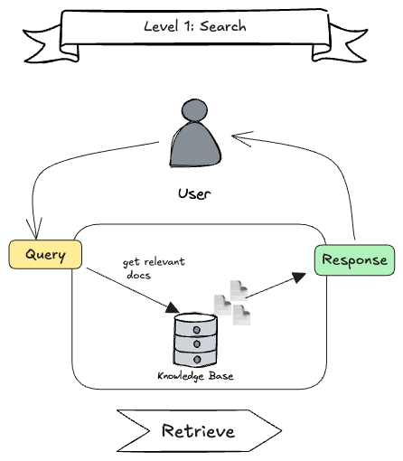
Level 1: Classic Search

While this is not RAG, it serves as the common ground where how traditional and simple retrieval systems can be designed. The user sends a query, the system looks for relevant documents in a knowledge base and returns them as a response. This is the pure “retrieval” step, no LLM involved.

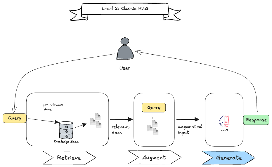
Level 2: Classic RAG

This is the classic RAG pattern, where the system retrieves relevant documents, augments the context with them, and then generates a response using an LLM. As we are on level 2, we only incorporate a single LLM call (blue box) , in this case to generate the output. All the other steps are known ahead of time making it a linear process that is easy to grasp. In many cases, the knowledge base is a vector database, but it can also be a keyword-based search or any other retrieval mechanism.

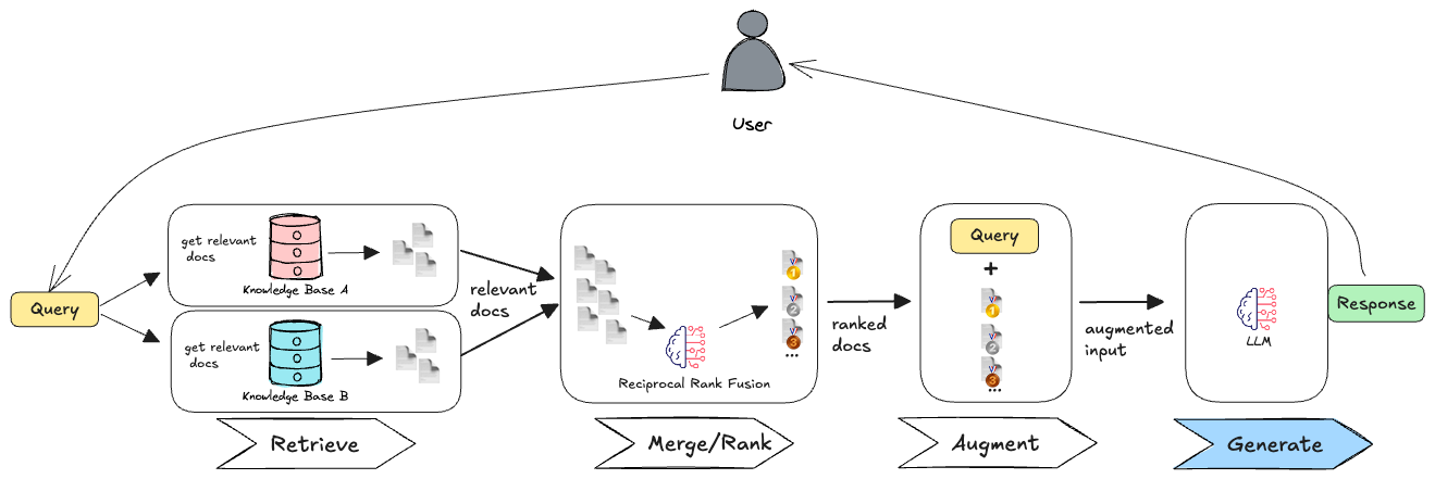
Also querying multiple knowledge bases in parallel is still considered a level 2 RAG technique, as we do not introduce any additional LLM calls to improve the retrieval process. The LLM is only used to generate the final response based on the retrieved documents. This is shown in the figure below, where we retrieve documents from two different knowledge bases and then generate a response based on the combined context (e.g. by using reciprocal rank fusion (RRF)).

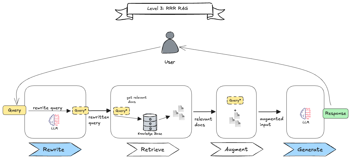
Level 3: Chained RAG

Here we introduce multiple LLM calls (blue boxes) to improve the system’s capabilities. There are many RAG implementations are implemented this way, for example:

Rewrite-Retrieve-Read (RRR): The initial query is rewritten to improve its quality to hopefully retrieve relevant documents (Figure 5).

Rerank RAG: After retrieving documents, we can rerank them based on their relevance to the query. This can be done by using a second LLM call to score the documents or by using a separate ranking model (Figure 6).

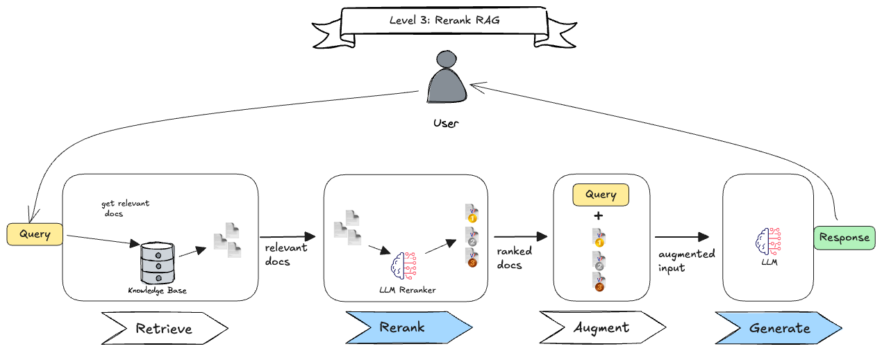
Hypothetical Document Embeddings (HyDE) : This technique generates hypothetical document embeddings based on the query and then retrieves documents that are similar to these embeddings. This can be used to improve the retrieval quality by generating embeddings that are more relevant to the query.

Of course, nobody stops you from combining the techniques above: Rewrite the query, retrieve documents from multiple knowledge bases, and then rerank them before generating the final response. From an architectural perspective, this is still a linear process, as you know every step and when it will be run a priori.

Level 4: RAG with Routers

On level 4, LLMs take over parts of the control flow and decide which step to take next based on the input and context. This allows for more dynamic and adaptive RAG systems, where the LLM can choose taking additional steps to improve results retrieval technique or decide whether to rerank documents or not.

In the example below (Figure 7), the corrective RAG (CRAG) pattern is implemented. After retrieving documents, the LLM grades the documents with a score. If the documents fall below a certain threshold, a corrective step is taken by invoking a web search to find more relevant documents. This is the first time we see a LLM-powered router in action, as it decides whether to take the corrective step or not based on the retrieved documents’ quality.

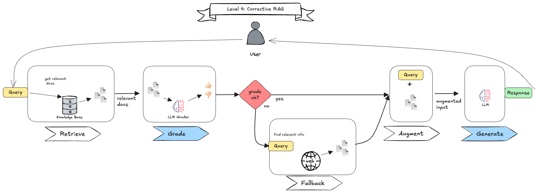
Note that we do not introduce cycles here, so it still represents a directed acyclic graph (DAG). You still know all the steps of this linear process and when they could be invoked, but the LLM decides whether to take them or not.

Level 5: RAG with State Machines

By adding cycles, these agentic RAG techniques can perform reflexive actions by observing and evaluating the results of previous steps, and then deciding whether to take corrective actions or not. Then it can restart (parts of) the process until a certain outcome is achieved. A rather complex example is Self-RAG (Figure 8), that leverages three grading steps (routers) to check for relevant documents, a grounded response and the usefulness w.r.t. to the question.

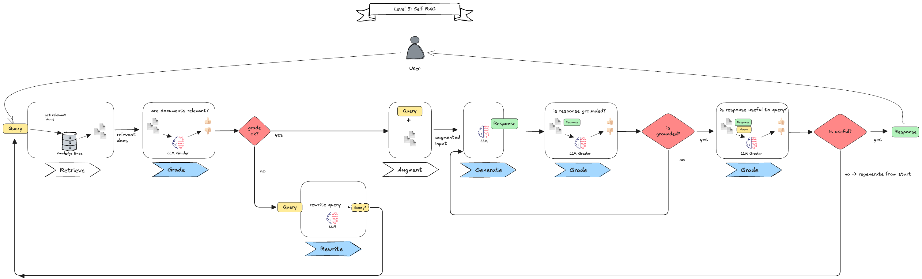
Taking a look at this architecture, we can see how many parts of the process are controlled by the LLM. This allows a more adaptive system, but the complexity also increases. Using structured responses and having a proper tracing in place are crucial to reason about the system’s behavior and to debug it when things go wrong.

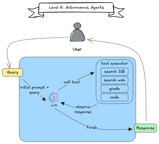
Level 6: Autonomous RAG Agents

One might think that a RAG technique on level 6 must be so complex that it cannot fit on the screen, when we take a look at the previous example. But in fact, the base is quite simple: The LLM is given an instruction and a set of tools (for example retrieval techniques) and can then decide which steps to take. This means, that we do not know ahead of time, which steps will be taken, how many times they will be invoked, and in which order. To fully fulfill the autonomy level 6, the LLM should also be able to refine its instruction and add new tools to its arsenal. One super interesting approach for this is CodeAct, which allows LLMs to write and execute code on the fly. Applied to our use case, it could write a new retrieval technique based on the user’s needs and then use it to retrieve relevant documents 🤯.

The right tool for the job 🔨

Does this mean that we should always strive for the highest autonomy level? Not necessarily. While higher autonomy levels can lead to more adaptive and powerful systems, they also come with increased complexity, unpredictability, and potential for failure. Especially when dealing with large amount of rather static data, a simpler RAG technique might be more suitable. In general, it is advised to use deterministic and less autonomous approaches the more you know the workflow in advance.

Simple Agents?

On the other hand people building coding agents report, that an agent equipped with retrieval tools like can outperform more complex systems that rely on advanced vector embeddings and indices. It also has been shown that for deep research contexts, a simple combination of keyword search like BM25 and an agent can achieve on par results compared to complex RAG systems, while having low inference and low storage requirements costs and complexity. This breaks with common beliefs that large volume of data requires complex vector embeddings for an agentic use case.

Conclusion

In the evolving landscape of AI, cognitive architecture patterns provide a structured approach to design and compare LLM-powered systems. From simple code to complex autonomous agents, each level of autonomy offers its own advantages and challenges. While more autonomy brings more complexity, it also opens doors to adaptive and powerful systems that can reason, plan, and execute tasks in ways that were previously unfeasible. As with nearly any topic in software architecture, there is no one-size-fits-all solution. Start with the simplest architecture that meets your needs, scaling autonomy only when tasks require dynamic decision-making.

An interesting trend is the rise of Agentic RAG, which combines the power of retrieval with the flexibility of agents. Especially when taking into account the rise of Model Context Protocol (MCP), new datasources and tools can be added on the fly, allowing agentic systems to adapt to new requirements without the need for complex redesign or reconfiguration. What we are particularly excited about is the potential of simple tools like keyword search to be used effectively in Agentic systems, proving that sometimes simple tools, wielded wisely, amplify its power.

Resources

Papers: